This article demonstrates how to fit a spatio-temporal dynamic
generalized linear model (STDGLM) to simulated data using the
STDGLM package. First, we load the required packages.
packages <- c("dplyr", "ggplot2", "tidyr", "ggpubr", "coda", "sf")

for (package in packages) {
  if (!require(package, character.only = TRUE)) {
    install.packages(package)
    require(package, character.only = TRUE)
  }
}
#> Loading required package: dplyr
#>
#> Attaching package: 'dplyr'
#> The following objects are masked from 'package:stats':
#>
#>     filter, lag
#> The following objects are masked from 'package:base':
#>
#>     intersect, setdiff, setequal, union
#> Loading required package: ggplot2
#> Loading required package: tidyr
#> Loading required package: ggpubr
#> Loading required package: coda
#> Warning in library(package, lib.loc = lib.loc, character.only = TRUE,
#> logical.return = TRUE, : there is no package called 'coda'
#> Installing package into '/home/runner/work/_temp/Library'
#> (as 'lib' is unspecified)
#> Loading required package: coda
#> Loading required package: sf
#> Linking to GEOS 3.12.1, GDAL 3.8.4, PROJ 9.4.0; sf_use_s2() is TRUE
Data Generation
The following chunk generates some covariates. We randomly sample
p=30 spatial locations within the unit
square. At these locations, we generate J=3 covariates (X) whose effects
vary in spacetime, the first one being an intercept, and q=1 covariate (z) whose effect
is held constant.
p = 30
set.seed(123)
coords = data.frame(x = runif(p), y = runif(p))
D = as.matrix(dist(coords))
t = 100
J = 3
X = array(1, dim = c(p, t, J))
for (j in 2:J) {
  for (t_ in 1:t) {
    set.seed(j*t_)
    X[, t_, j] = rnorm(p)
  }
}
q=1
set.seed(10)
z = array(rnorm(p*t*q), dim = c(p, t, q))
Then we simulate some varying coefficients and plot them.
beta0 <- outer(
  seq(0.7, 1.5, length.out = p),
  -10*(seq(0,1,length.out = t)-0.5) - 50*(seq(0,1,length.out = t)-0.5)^2 + 10
)

tempo <- (1:t)
beta1 <- outer(
  - .6* (coords$x-.9)^2 + .6* (coords$y-.5)^2,
  sin(tempo/t*2*pi) + 3, FUN = "+"
)

beta2 = 4*outer(
  - .6* (coords$x-.9)^2 + 1* (coords$y-.5)^2,
  0.5*sin(tempo/t*2*pi) + 0.5*cos(tempo/t*4*pi),
  FUN = "+"
)


Next, we simulate the response variable Y using the
observation equation. The observation error is assumed to be normally
distributed with mean zero and variance \sigma_\epsilon^2 = 2.
gamma <- 1
set.seed(42)
eps = matrix(rnorm(p*t, sd = sqrt(2)), nrow = p, ncol = t)
Y <- beta0 + beta1*X[,,2] + beta2*X[,,3] + gamma*z[,,1] + eps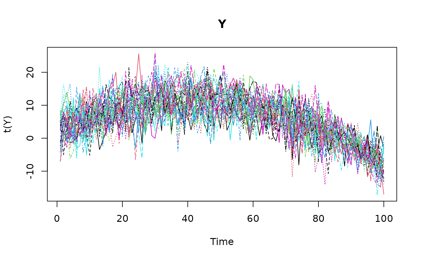
Model Fitting
Before fitting the model, we need to prepare a list of prior
hyperparameters. Here, we assume vague priors for all the parameters.
These are also the default values used when prior=NULL.
prior_list = list(
  V_beta_0 = 1e4,         # Prior variance of initial state
  V_gamma = 1e6,          # Prior variance of constant coefficients
  a_inn_time = 0.01,      # Prior shape for temporal variance
  b_inn_time = 0.01,      # Prior rate for temporal variance
  a_rho1s = 0.01,         # Prior shape for spatial variance
  b_rho1s = 0.01,         # Prior rate for spatial variance
  a_rho1st = 0.01,        # Prior shape for spatio-temporal variance
  b_rho1st = 0.01,        # Prior rate for spatio-temporal variance
  s2_a = 0.01,            # Prior shape for measurement error variance
  s2_b = 0.01             # Prior rate for measurement error variance
)
The MCMC setup is provided in the next chunk. You can adjust the
number of iterations, burn-in period, thinning interval, and other
parameters as needed. The point.referenced argument
indicates that the data are point-referenced, and
random.walk specifies that we want to use a random walk
structure for time-varying parameters.
nburn <- 200                # burn-in period
nrep <- 200                 # number of iterations to save after burn-in
thin <- 1                   # thinning interval
point.referenced = TRUE     # data are point-referenced
random.walk = TRUE          # random walk structure for time-varying parameters
print.interval = 50         # print message during execution of MCMC
The following command executes the MCMC algorithm to fit the STDGLM
model to the simulated data. The stdglm function takes the
response variable Y, covariates X and
z, and other parameters defined above. The output is an
object of class stdglm, i.e. a list containing the MCMC
samples and other posterior summaries. The output is described in a
separate article.
mod <- stdglm(y=Y, X=X, Z=z,
              point.referenced=point.referenced,
              random.walk=random.walk,
              W=D,
              nrep=nrep, nburn=nburn, thin=thin,
              print.interval=print.interval,
              prior=prior_list
)
#> Starting MCMC (400 iterations)...
#> Iteration: 50 / 400
#> Iteration: 100 / 400
#> Iteration: 150 / 400
#> Iteration: 200 / 400
#> Iteration: 250 / 400
#> Iteration: 300 / 400
#> Iteration: 350 / 400
#> Iteration: 400 / 400
#> MCMC finished.
fitted, coef and plot
methods
The fitted method provides the mean of the posterior
predictive distribution for the observed data points. We can also
plot the fitted values against the observed data for a
specific location.
fitted_values <- fitted(mod)
print(dim(fitted_values))
#> [1]  30 100
summary(t(fitted_values[1:5,]))
#>        V1                V2               V3                V4
#>  Min.   :-8.0731   Min.   :-8.794   Min.   :-10.041   Min.   :-12.383
#>  1st Qu.: 0.4735   1st Qu.: 1.875   1st Qu.:  2.092   1st Qu.:  0.539
#>  Median : 4.3935   Median : 5.713   Median :  5.392   Median :  6.080
#>  Mean   : 3.9990   Mean   : 4.886   Mean   :  4.699   Mean   :  5.044
#>  3rd Qu.: 6.9766   3rd Qu.: 8.587   3rd Qu.:  7.949   3rd Qu.:  9.050
#>  Max.   :16.5299   Max.   :13.997   Max.   : 14.391   Max.   : 16.155
#>        V5
#>  Min.   :-11.581
#>  1st Qu.:  1.693
#>  Median :  4.749
#>  Mean   :  4.766
#>  3rd Qu.:  8.407
#>  Max.   : 19.634
plot(mod, Y=Y, id=1) # pick a number between 1 and p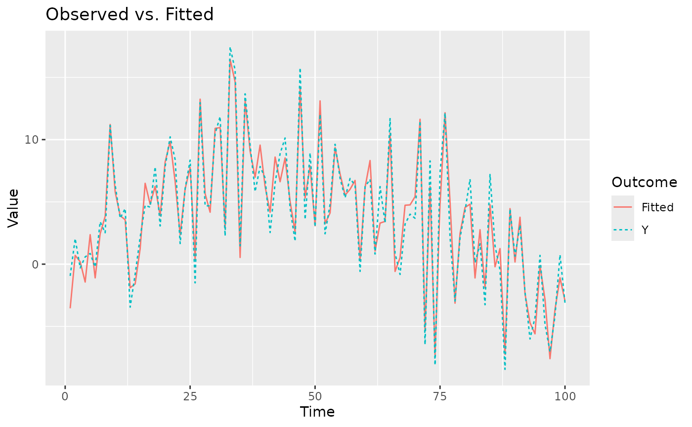
The plot method returns an object from the
ggplot2 package, so it is straightforward to customize,
save, and arrange multiple plots.
g1 = plot(mod, Y=Y, id=1)
# ggsave("plot1.png", plot = g1)
g2 = plot(mod, Y=Y, id=2)
# ggsave("plot2.png", plot = g2)

ggarrange(g1, g2, labels = c("#ID 1", "#ID 2"), label.x = 0.8)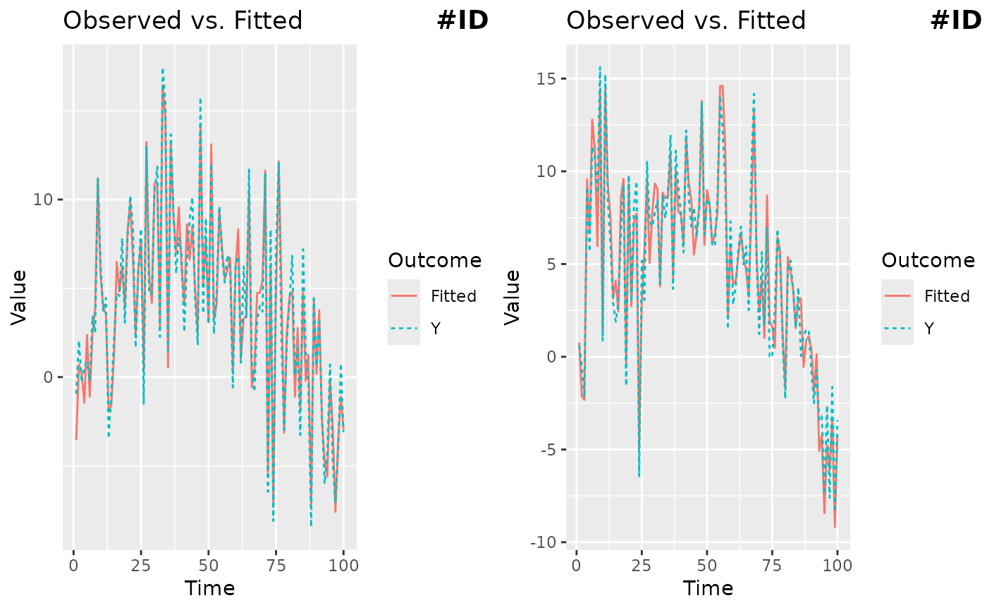
Posterior summaries for all the coefficients can be extracted using
the coef method. Here we show those of constant
coefficients.
print(coef(mod, 'overall'))
#> Mean sd ci_low ci_high
#> 1 6.3168361 0.02767138 6.2626011 6.37107097
#> 2 2.9331528 0.02717265 2.8798954 2.98641022
#> 3 -0.1092179 0.02771084 -0.1635301 -0.05490561
print(coef(mod, 'gamma'))
#> Mean sd ci_low ci_high
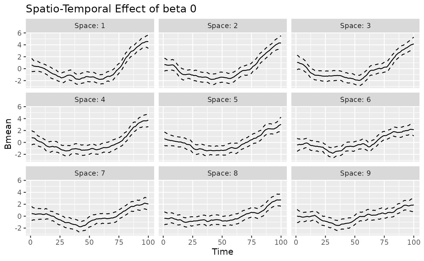
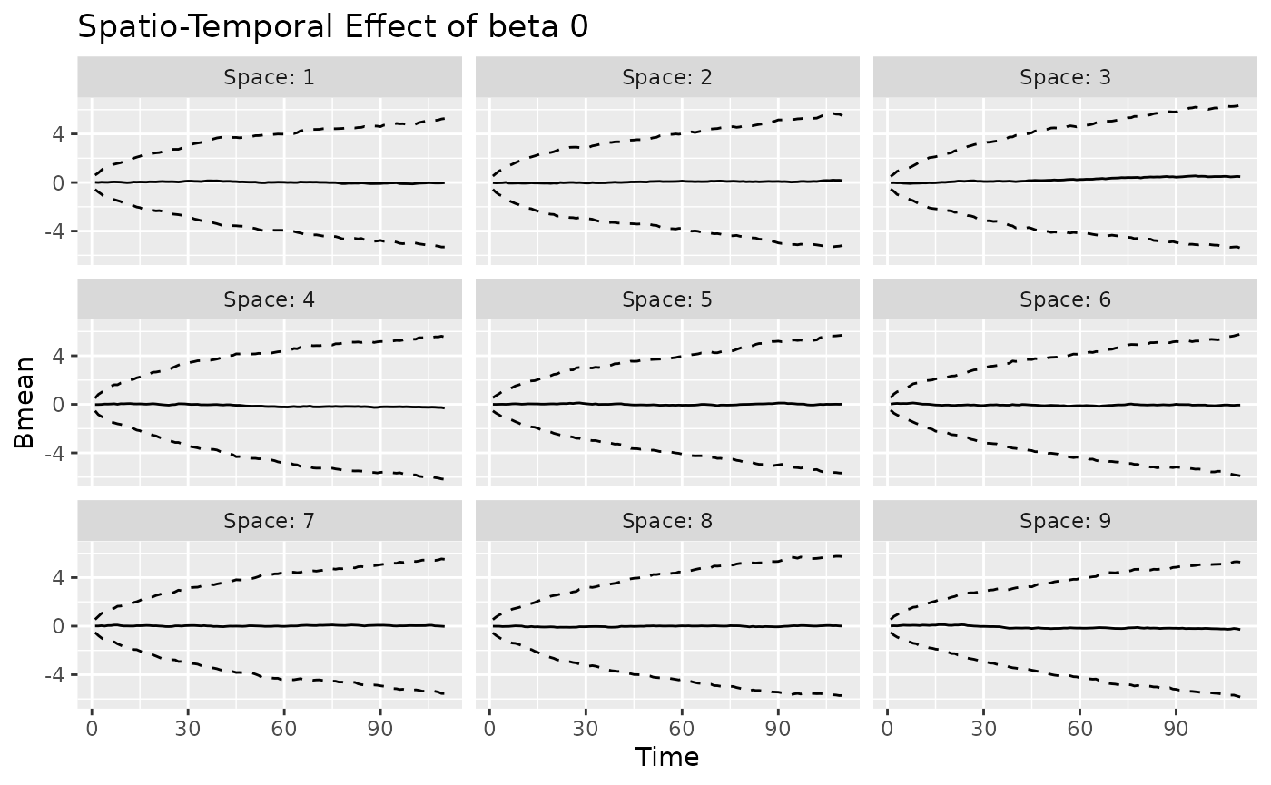
#> 1 1.006071 0.02622202 0.9546773 1.057466The plot method can also be used to visualize the
time-varying, space-varying, and spacetime-varying coefficients. The
returned object is a ggplot object. The label “Observed”
indicates that the values refer to the observed spatio-temporal data
points. For time-varying and spacetime-varying coefficients, the 95%
credible intervals (CI) are within the dashed lines, whereas for the
space-varying coefficients the posterior standard deviation is shown for
each location.
plot(mod, 'tvc')
#> [[1]]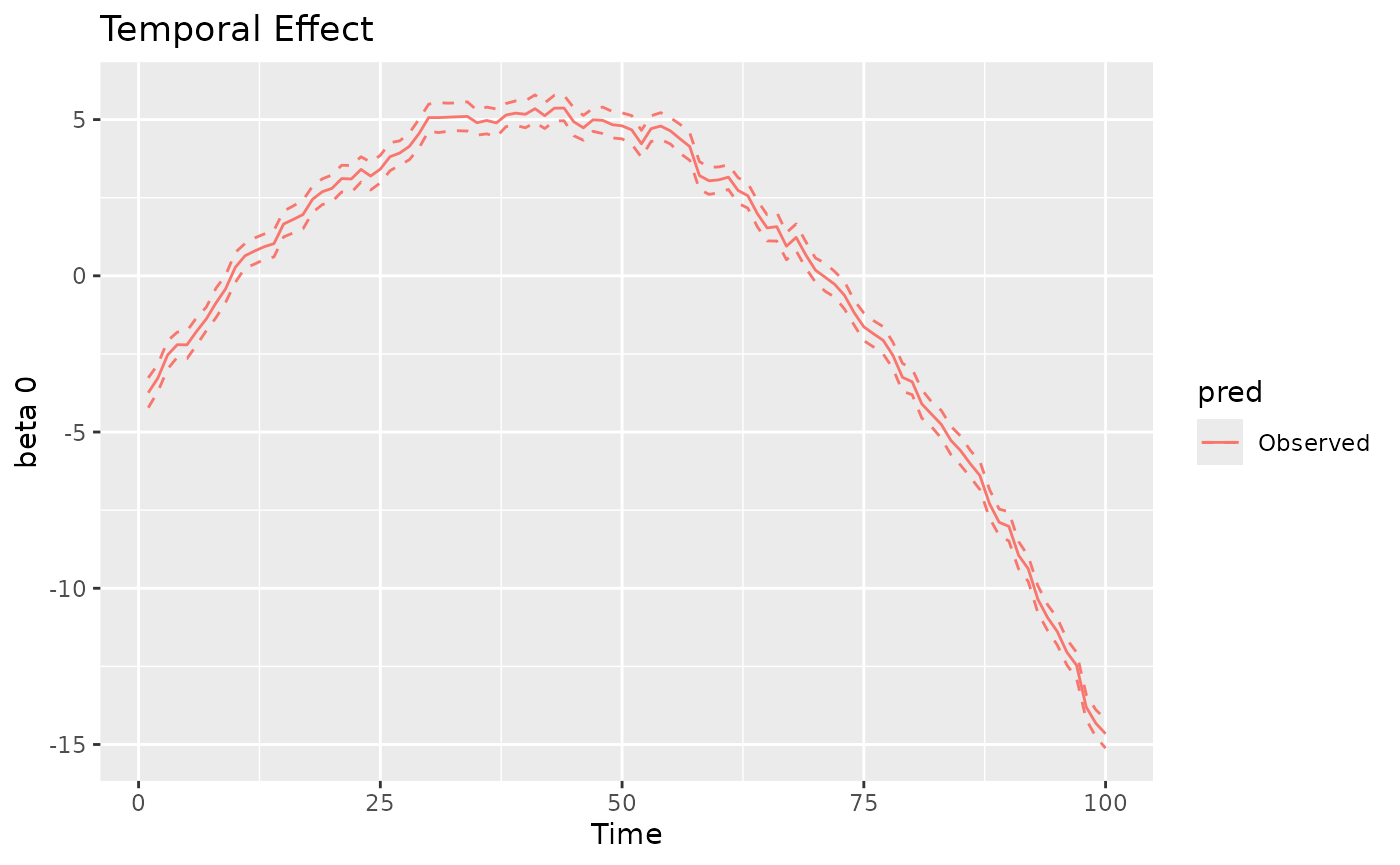
#>
#> [[2]]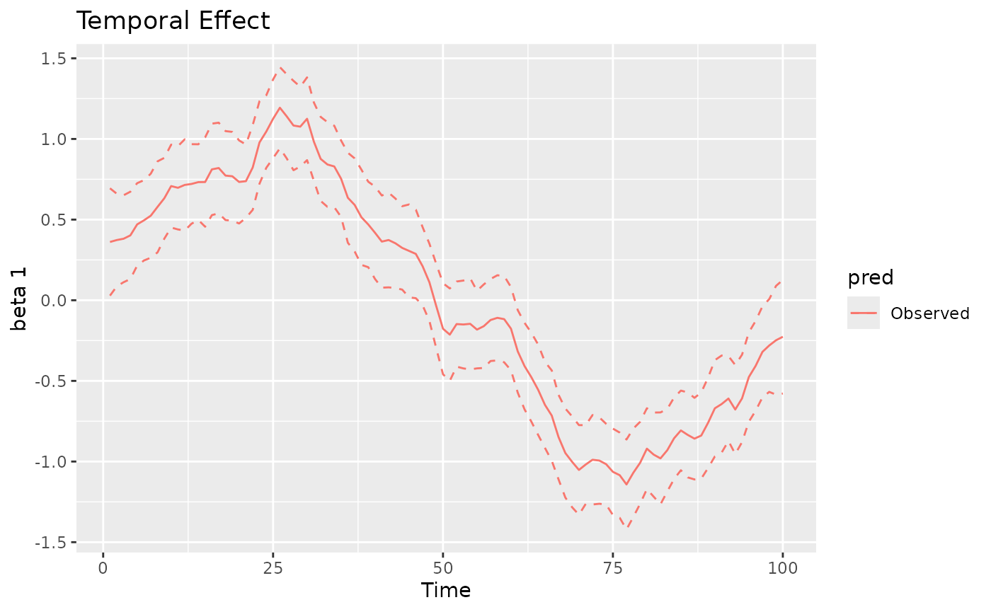
#>
#> [[3]]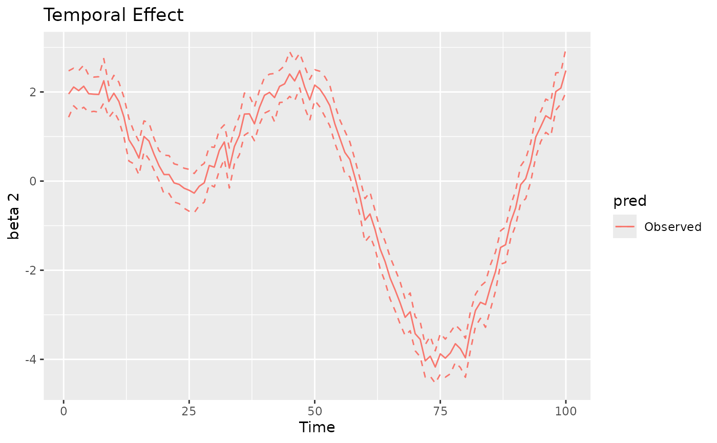
coords_sf = st_as_sf(coords, coords = c("x", "y"))
unit_square_coords <- matrix(
  c(
    0, 0,
    1, 0,
    1, 1,
    0, 1,
    0, 0
  ),
  ncol = 2,
  byrow = TRUE
)
region = st_sf(
  geometry = st_sfc(st_polygon(list(unit_square_coords)))
)
plot(mod, 'svc', coords_sf, region)
#> [[1]]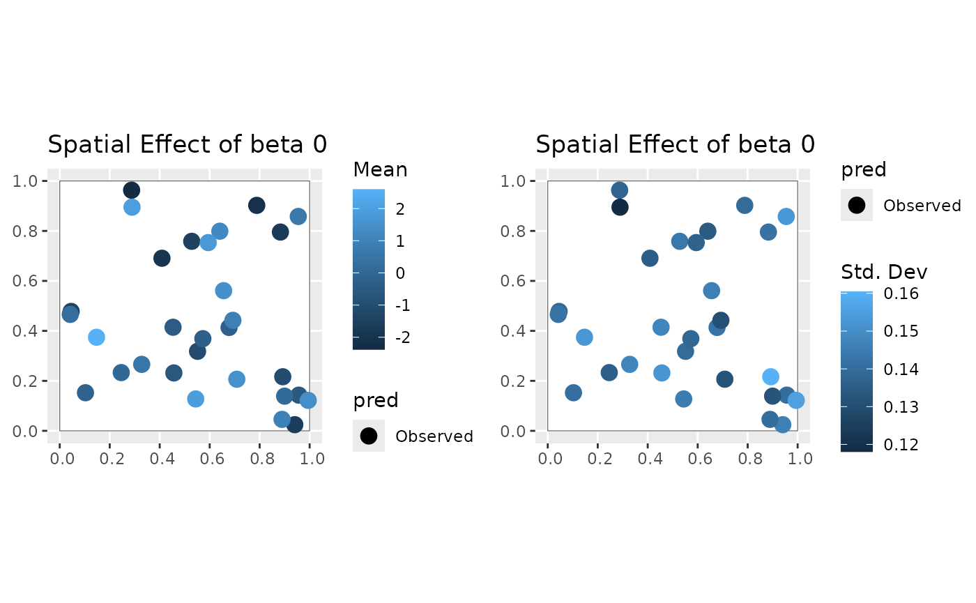
#>
#> [[2]]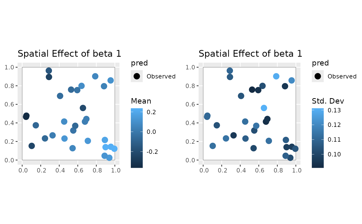
#>
#> [[3]]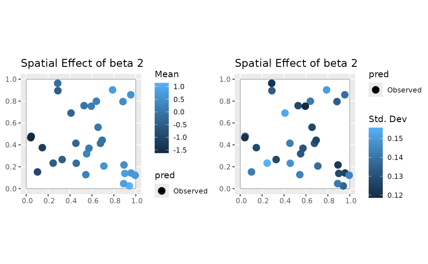
#>
#> [[2]]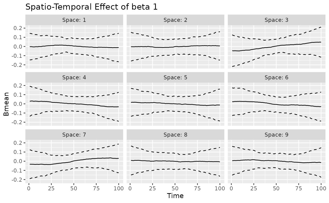
#>
#> [[3]]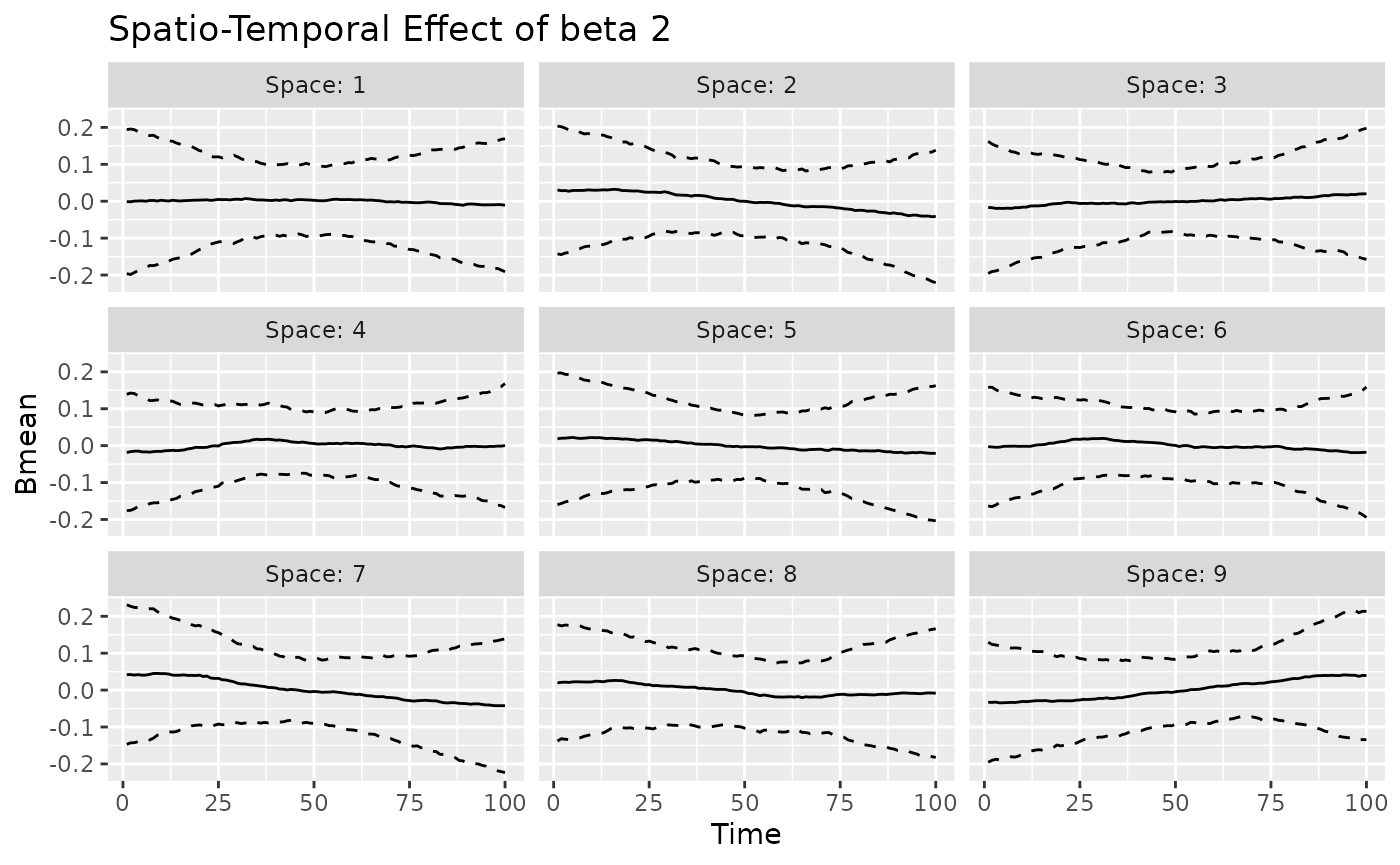
The coef method can be used also for the varying
coefficients. For example, we can compare the posterior mean of the
spacetime-varying effect of beta0 with its true value.
st_effect_b0 = beta0 + mean(beta0) -
  matrix(rowMeans(beta0), nrow = nrow(beta0), ncol = ncol(beta0)) -
  matrix(colMeans(beta0), nrow = nrow(beta0), ncol = ncol(beta0), byrow = TRUE)

beta0_post = coef(mod, 'stvc') %>%
  filter(Coef == 'beta0') %>%
  mutate(Truth = as.vector(st_effect_b0)) %>%
  filter(Space %in% 1:9) %>%
  select(Space:Mean, Truth) %>%
  pivot_longer(cols = c('Mean', 'Truth'), names_to = 'Type', values_to = 'Value')
ggplot(beta0_post, aes(x = Time, y = Value, color = Type)) +
  geom_line() +
  facet_wrap(~ Space, nrow = 3) +
  labs(title = "Posterior Mean vs Truth for beta0")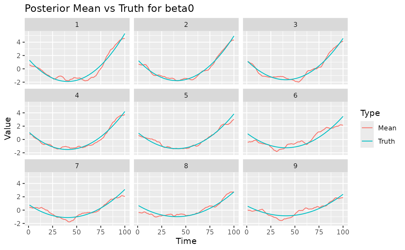
Trace plots
We can also visualize the trace plots of the MCMC samples for the
parameters of interest. For that purpose, we can convert the output to
an mcmc object, then use the plot function
from the coda package.


if (!random.walk) {
  plot(mcmc(t(mod$out$phi_AR1_time))) # AR(1) coefficient for temporal evolution for j=1,...,J
  plot(mcmc(t(mod$out$phi_AR1_spacetime))) # AR(1) coefficient for spatio-temporal evolution for j=1,...,J
}
plot(mcmc(t(mod$out$gamma))) #  coefficient of the z covariate
Restoring previous state
The MCMC algorithm has not converged yet, however it is very easy to
continue previous chain. You just need to provide mod as an
argument to the stdglm function. The MCMC will continue
from the last saved state. Note that all previous samples will be
discarded.
mod <- stdglm(y=Y, X=X, Z=z,
              point.referenced=point.referenced,
              random.walk=random.walk,
              W=D,
              nrep=nrep, nburn=nburn, thin=thin,
              print.interval=print.interval,
              prior=prior_list,
              last_run = mod
)
Model Selection and Comparison
The stdglm object also contains tools for model
selection and comparison, including the Deviance Information Criterion
(DIC), the Widely Applicable Information Criterion (WAIC), scoring rules
and Bayesian p-values. These are all described in a
separate article.
Temporal predictions and Spatial interpolation
In this section, we will demonstrate how to perform out-of-sample
predictions. We will create a grid of new spatial locations and generate
new covariates for these locations. We also assume that we want to
predict the next 10 time points, so we set h_ahead = 10.
The new covariates are generated in a similar way as before, but now we
have p_new locations and t_new = t + h_ahead
time points.
st_new = st_make_grid(region, what = "centers", n = c(20, 20))
p_new = NROW(st_new)
h_ahead = 10
t_new = t + h_ahead

coords_pred = as.data.frame(st_coordinates(st_new))
names(coords_pred) = names(coords)

Xpred = array(1, dim = c(p_new, t_new, J))
for (j in 2:J) {
  for (t_ in 1:t_new) {
    set.seed(j*t_*2)
    Xpred[, t_, j] = rnorm(p_new)
  }
}

q=1
set.seed(10*8)
zpred = array(rnorm(p_new * t_new * q), dim = c(p_new, t_new, q))
The function stdglm performs spatial interpolation using
a blocked structure. This is useful when the number of new spatial
locations is very large. Therefore, three lists are created to store the
indices of new locations (blocks_indices), the distance
matrices for the prediction locations (D_pred), and the
cross-distance matrices (D_cross). In the following code
chunk, each block is made up of just one location.
ii = floor(seq(1, p_new+1, by = 1))
lii = length(ii)

D_pred = D_cross = blocks_indices = vector('list', lii-1)
for (i in 2:lii) {
  Dalltemp = as.matrix(dist(rbind(coords, coords_pred[ii[i-1]:(ii[i]-1), ])))
  D_pred[[i-1]] = unname(Dalltemp[-(1:p), -(1:p), drop=FALSE])
  D_cross[[i-1]] = unname(Dalltemp[1:p, -(1:p), drop=FALSE])
  blocks_indices[[i-1]] = ii[i-1]:(ii[i]-1)
}
The following command fits the STDGLM model, continuing the previous
run. There is also the possibility to set the number of cores for
parallel processing using the ncores argument: if its value
is greater than 1, the spatial predictions will be performed in parallel
during each MCMC iteration.
mod <- stdglm(y=Y, X=X, Z=z,
              point.referenced=point.referenced,
              random.walk=random.walk,
              blocks_indices=blocks_indices,
              W=D, W_pred=D_pred, W_cross=D_cross,
              X_pred=Xpred, Z_pred=zpred,
              ncores = 1, # Set number of cores for parallel processing
              nrep=nrep, nburn=nburn, thin=thin,
              print.interval=print.interval,
              prior=prior_list,
              last_run = mod
)
#> Restarting MCMC from previous state...
#> Starting MCMC (400 iterations)...
#> Iteration: 50 / 400
#> Iteration: 100 / 400
#> Iteration: 150 / 400
#> Iteration: 200 / 400
#> Iteration: 250 / 400
#> Iteration: 300 / 400
#> Iteration: 350 / 400
#> Iteration: 400 / 400
#> MCMC finished.
The plot method can be used again to visualize the
posterior predictive summaries (posterior mean and 95% CIs) of the
varying coefficients. The observed spatio-temporal points are clearly
distinguished from the predicted ones.
plot(mod, 'tvc')
#> [[1]]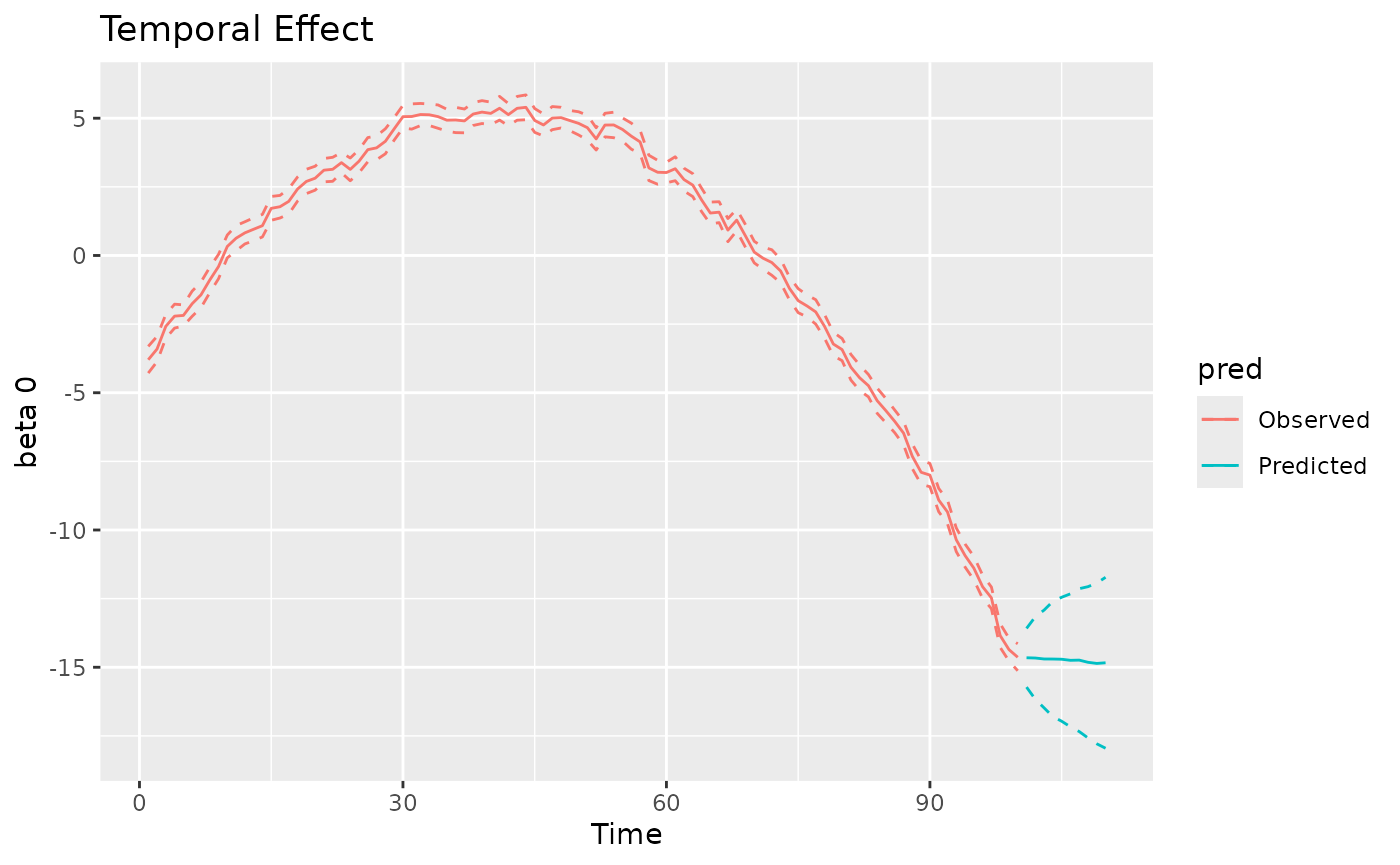
#>
#> [[2]]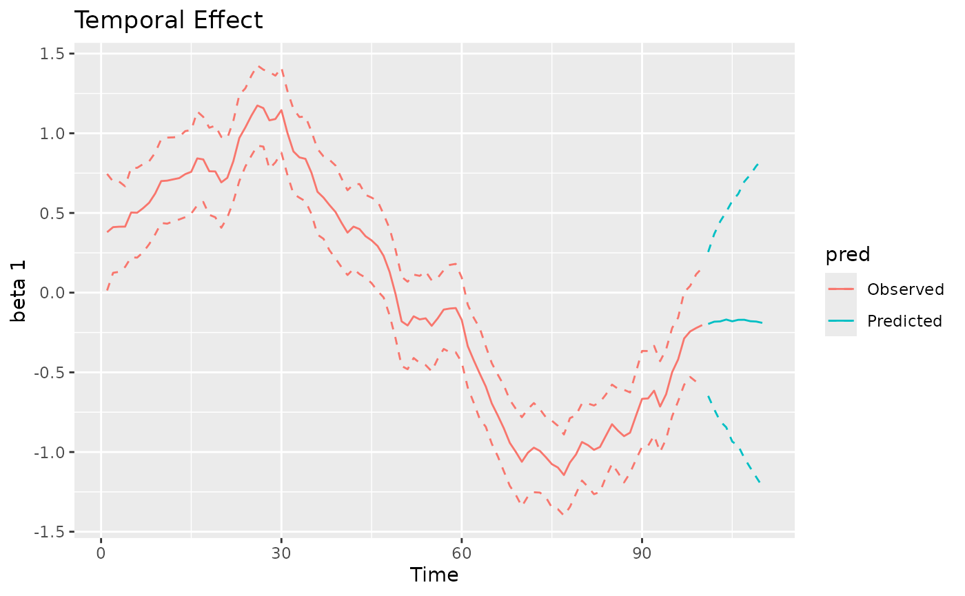
#>
#> [[3]]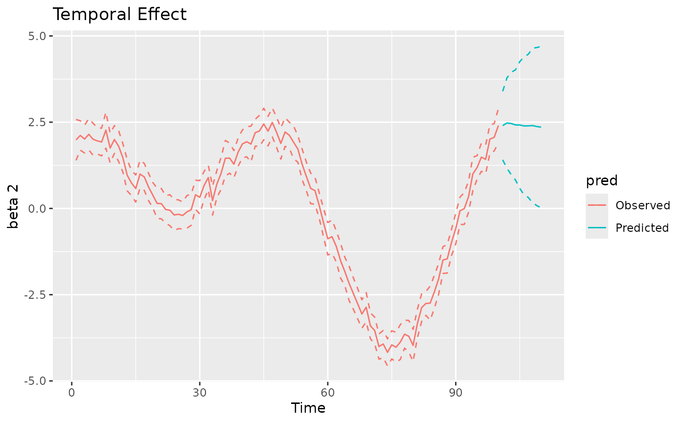
coords_pred_sf = st_as_sf(coords_pred, coords = c("x", "y"))
plot(mod, 'svc', coords_sf, region, coords_pred_sf)
#> [[1]]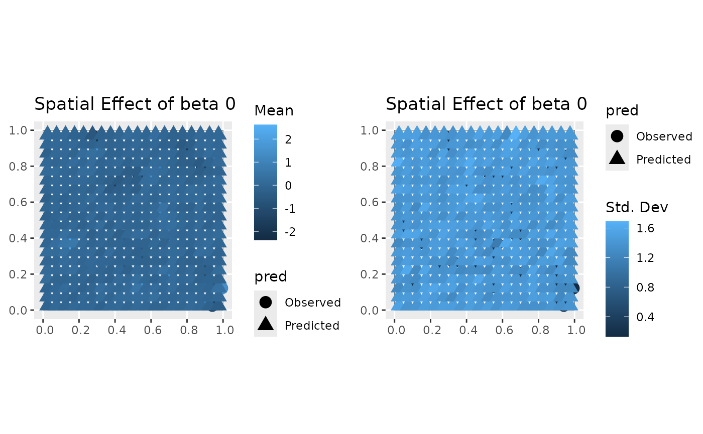
#>
#> [[2]]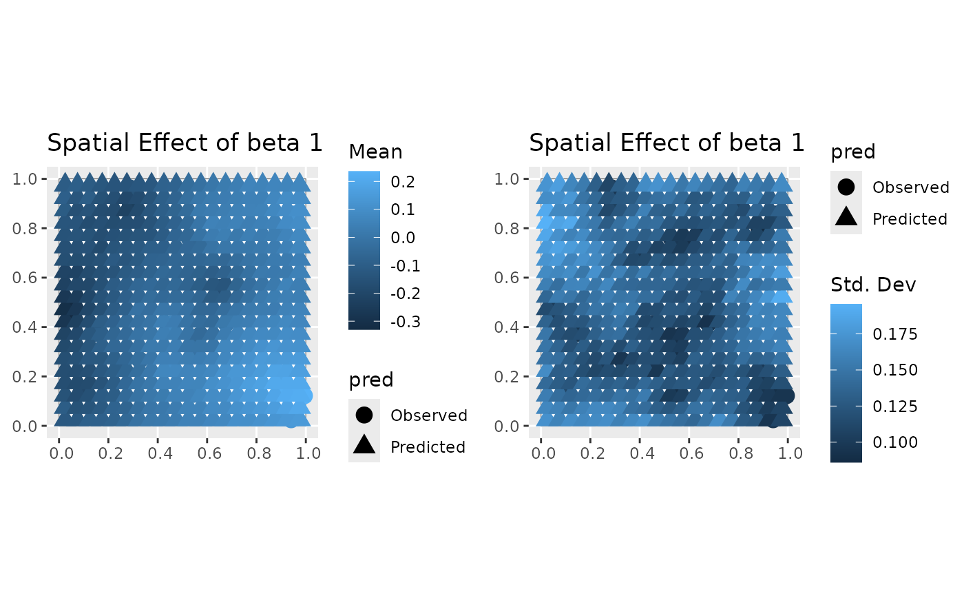
#>
#> [[3]]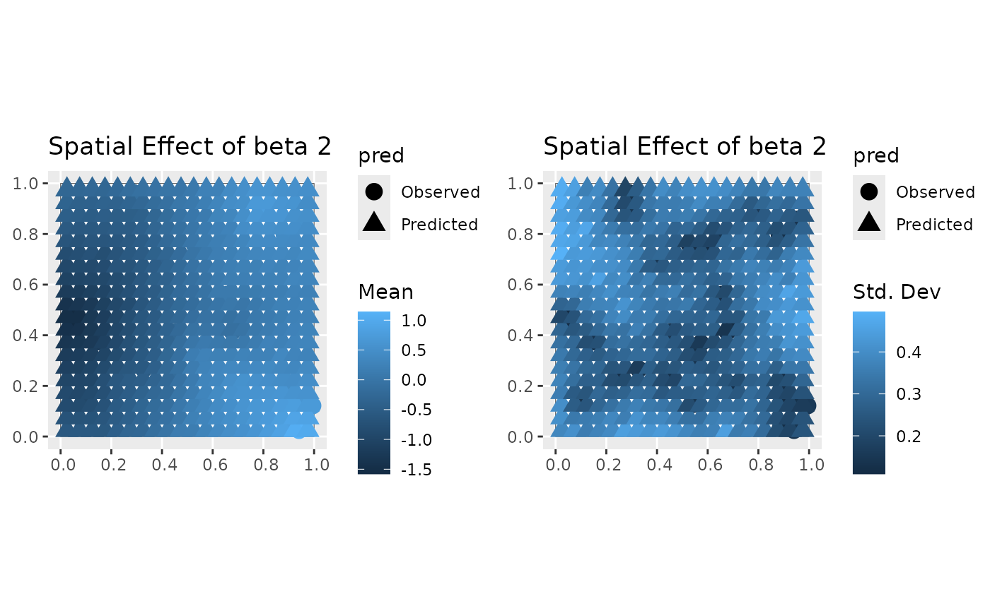
#>
#> [[2]]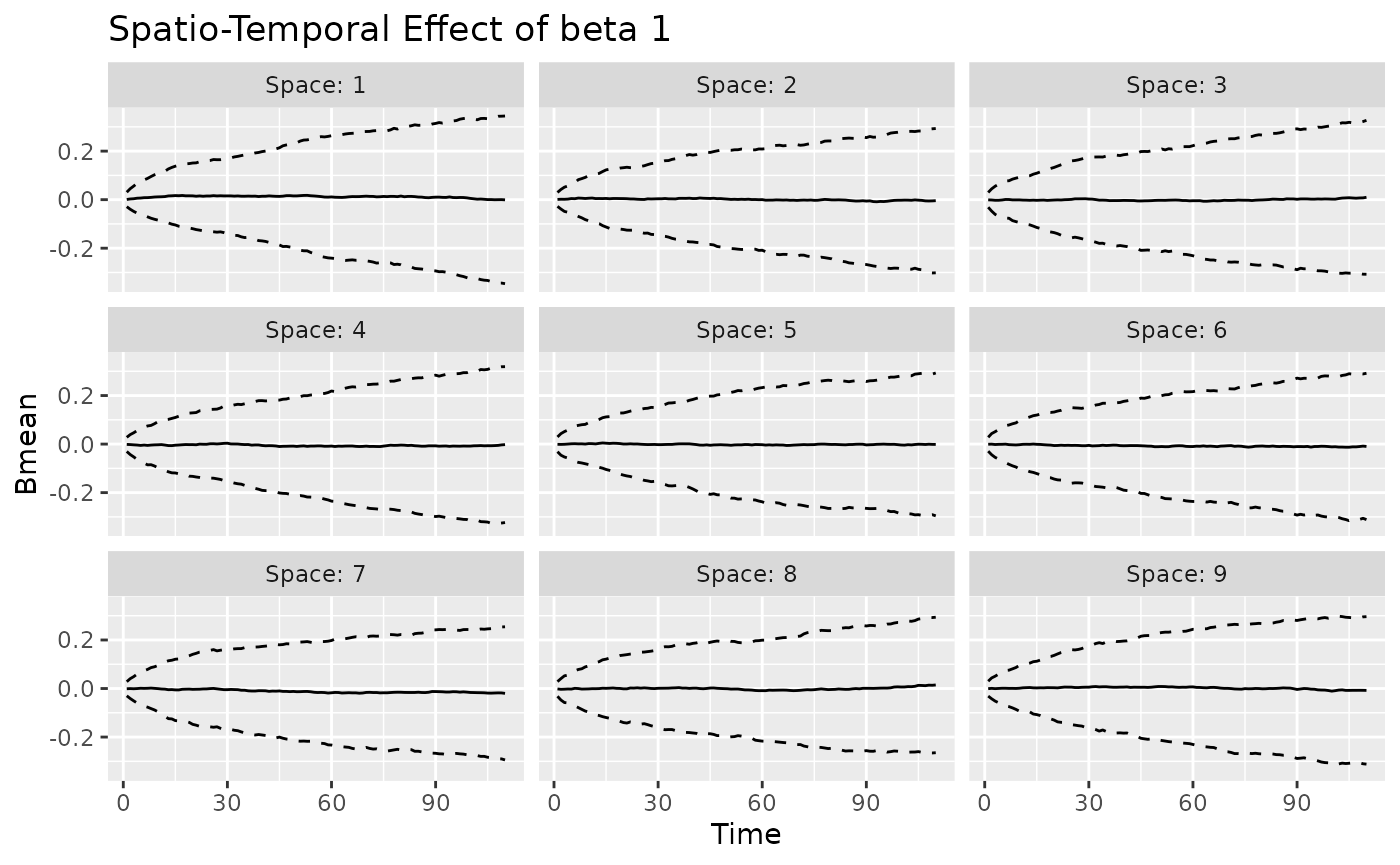
#>
#> [[3]]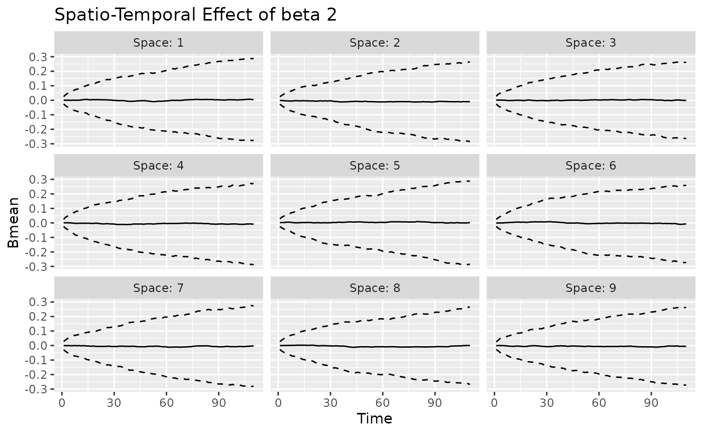
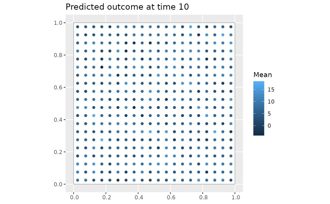
The predict method can be used to easily access the
posterior predictive summaries, for both the response variable, as shown
below, and the varying coefficients. The input Coo_sf_pred
(optional) allows to return a simple feature object, which may be useful
for plotting.
Y_pred = predict(mod, type = 'response_df', Coo_sf_pred = coords_pred_sf)
ggplot(Y_pred %>% filter(Time==10)) +
    geom_sf(data = region, fill = "white") +
    geom_sf(aes(color = Mean)) +
    labs(title = "Predicted outcome at time 10")